I’m a fan of code abstraction; I like how clean code looks and “feels”. I think that clean and good code is like art. And just like art can be categorized into styles such as Impressionism, Neo-Impressionism, and Post-Impressionism (all of which I like), we can also organize code.
In this post, I do not talk about functional vs. imperative vs. object-oriented programming but the mathematical structure in code. You might have heard of concepts such as monads, monoids, functors, etc. At an abstract level, these concepts lay out specific properties that we can use to describe how data can flow between various classes (in the programming sense, e.g., python, c++, java, etc.). The benefit here is that if your code fulfills the requirements laid out by these categories, you get certain guarantees about your program regarding results and how you can compose them together.
This is the first in a series of blog posts discussing categories in programming languages that hopefully help you notice patterns to write cleaner code. This series will not be mathematical and assumes no prior knowledge other than python (which you don’t even really need - it just provides a concrete example of what we’re doing).
We will continually expand on the following scenario throughout the series as we go from “ugly” unabstracted code to clean abstractions. It’s important to note that you (and I) have probably written code that fits into these concepts without even realizing it! The concepts introduced here are to make you more aware of what you are writing and make you notice these patterns, allowing you to reuse lots of code you have already written.
1) Initial Project
You are working on a project involving “parallel” computation, e.g., you have multiple computers or processes on the same system. Concretely, you have 100 machines with identical datasets on them. You want to do a hyperparameter search, e.g., ten searches over each of the 100 machines, totaling 1K runs. For each run, you want to track some validation loss before returning the model with the lowest validation loss.
Note: Throughout this post we assume that you have some train and validate method implemented.
1.1) Simple Scenario
If you were to find the best model, you might have something like the following:
Dataset = Tuple[NumericalArray, NumericalArray]
ValidationResults = List[float]

def Node(object):
    """
    A compute node on a single machine
    """
    def __init__(self, data: Dataset, hyperparameters: Dict[str, Any]):
        self.train_data = data[0]
        self.validation_data = data[1]
        self.conf = hyperparameters
        self.validation_losses = []

    def run(self):  # A Map
        """Run the training and validation"""
        for conf in self.conf:
            trained_model = train(conf, self.train_data)
            self.validation_losses.append(validate(trained_model, self.validation_data))

    def report(self, validation_lists: List[ValidationResults]) -> float:  # A reduce
        """
        validation_lists = [
            [1, ..., 10]  # Node 1
            [0.1, ..., 1.0] # Node 2
            ....
        ]
        """
        minimum = math.inf
        for arr in validation_lists:
            minimum = min(minimum, min(arr))
        return minimum
And you would distribute this to all your nodes. After completing its computation, each node will send its report (a list of 10 floating numbers describing the validation loss) to a “reducer” node. The reducer node will accumulate all 1K results before reducing them to find the minimum value.
1.2) Complicated Scenario
The situation above is simple; the final node in the graph accumulates all the report results and finds the minimum, which is simple and doesn’t take up too much memory since floats are cheap to store.
However, what happens if we want to find more than just the minimum losses, and our data takes up much more memory? In this case, we would like to apply multiple reductions; Nodes 1-10 send their results to Reducer1, Nodes 11-20 send to Reducer2, and so forth. At the end, we have a final reducer which takes results from all the reducers for our final result
Our code now looks like the following:
Dataset = Tuple[NumericalArray, NumericalArray]
ValidationResults = List[float]
Data = Union[Dataset, ValidationResult]

def Node(object):
    """
    A compute node on a single machine which either:
        - runs the hyperparameter search
        - runs a reduction on the data
    """
    def __init__(self, data: Data, hyperparameters: Optional[Dict[str, Any]] = None):
        """
        In the case of our data being of instance `ValidationResults`, hyperparameters is an empty dictionary
        """

        # On our "reducer" nodes
        if isinstance(data, List):
            self.data = data
        else:
            self.train_data = data[0]
            self.validation_data = data[1]
        self.conf = hyperparameters

        self.validation_losses = []

    def run(self):
        """Run the training and validation"""

        # Our reduce step
        if hasattr(self, data):
            self.validation_losses = self.data
            return
        # Our map-and-run step
        for conf in self.conf:
            trained_model = train(conf, self.train_data)
            self.validation_losses.append(validate(trained_model, self.validation_data))

    def report(self) -> float:
        """
        All of the results here get collected and saved
        """
        return min(validation_losses)
1.2.1) Messiness
As we can see above, the code is quite messy. The messiness is because we have to care about the underlying data and what to do with it. We want to squint our eyes and abstract all the conditionals and checks.
Concretely, we would like to abstract away the values and make it cleaner, which we can do by the following:
class Dataset():
    def __init__(self, data: Tuple[NumericalArray, NumericalArray], hyperparameters):
        self.train_data = data[0]
        self.validation_data = data[1]
        self.conf = hyperparameters

        self.validation_losses = []

    def run(self):
        for conf in self.conf:
            trained_model = train(conf, self.train_data)
            self.validation_losses.append(validate(trained_model, self.validation_data))

    def report(self) -> float:
        return min(self.validation_losses)

class ValidationResults():
    def __init__(self, data: List[float], _: Optional[Any] = None):
        self.data = data

    def run(self):
        return

    def report(self) -> float:
        return min(self.data)

Container = Union[Dataset, ValidationResults]

def Node(object):
    """
    A compute node on a single machine which either:
        - runs the hyperparameter search
        - runs a reduction on the data
    """
    def __init__(self, container: Container):
        self.container = container

    def run(self):
        # The individual types handle their own run
        self.container.run()

    def report(self) -> float:
        # The individual types handle their own reduction
        return self.container.report()
As we can see, we defined two classes above, which will handle the run and report as necessary. By delegating the calls, we, as the programmer, do not have to care what the underlying Container is.
In my opinion, this is much cleaner! This way, we have decoupled the run logic from the underlying data type. All we need to do is call the appropriate values.
At a higher level, this is freeing because we can treat these class instances are abstract containers - as long as something follows the type-signatures of run and report from Node, it should, in theory, work out exactly as they expect.
1.2.2) So what?
However, none of this should be new to you. Creating an abstract interface to make code clean isn’t anything “interesting” in and of itself. Let’s go deeper.
2) The Second Phase
In the second phase of the project, you decide that you want to add in things like:
- running average
- standard deviation
- tracking the 100 best models in terms of validation losses
Which would ultimately derail the structure we’ve got above…. or would it? Let’s take a look at the custom types we have defined so far:
Dataset
- run
- report
ValidationResult
- run
- report
We notice that our Dataset doesn’t change much, other than the Dataset.run. Our ValidationResult will change, but that’s understandable.
Note In the following, I assume you’ll be keeping track of the top 100 best models in your own way. I’ll be “using” a heap, but I won’t include any logic for it because that’s not the point of this work.
2.1) Naive Approach
The naive approach (which would probably come to mind first) would be the following
P.s: at the end of our reduce step, we have a dictionary of values which we must process to get whatever values you want.
class Dataset():
    def __init__(self, data: Dataset = Tuple[NumericalArray, NumericalArray], hyperparameters):
        self.train_data = data[0]
        self.validation_data = data[1]
        self.conf = hyperparameters

        self.validation_losses = []


    def run(self):
        self.validation_loss_min_heap = heapify([])
        for conf in self.conf:
            trained_model = train(conf, self.train_data)
            validation_losses = validate(trained_model, self.validation_data)
            self.validation_losses.append(validation_losses)

            # you do the checks and logic
            self.validation_loss_min_heap.insert(validation_losses)


    def report(self) -> Dict[str, float]:
        return {
            "min": min(self.validation_losses),
            "sum": sum(self.validation_losses),
            "count": len(self.validation_losses)
            "best_100": self.validation_loss_min_heap
        }

class ValidationResultDict():
    def __init__(self, data: List[Dict], _):
        self.data = data

    def run(self):
        return

    def report(self):
        min_so_far = math.inf
        sum_so_far = 0
        count_so_far = 0
        validation_loss_min_heap = heapify([])
        for data_dict in self.data:
            min_so_far = min(min_so_far, data_dict["min"])
            sum_so_far = sum_so_far + data_dict["sum"]
            count_so_far = count_so_far + data_dict["count"]

            # you do the checks and logic
            validation_loss_min_heap.insert(data_dict["best_100"])

        return {
            "min": min_so_far
            "sum": sum_so_far,
            "count": count_so_far
            "best_100": validation_loss_min_heap
        }

Container = Union[Dataset, ValidationResult]

def Node(object):
    """
    A compute node on a single machine which either:
        - runs the hyperparameter search
        - runs a reduction on the data
    """
    def __init__(self, data: Data):
        self.container = data

    def run(self):
        # The individual types handle their own run
        self.container.run()

    def report(self) -> Dict:
        # The individual types handle their own reduction
        # Also, you now have to process the returned dictionary
        return self.container.report()
where we added custom code to track the state and update our dictionary container. However, as we can see, there is a LOT of similarity between the Dataset.report and ValidationDatasetDict.report. Can we make this cleaner?
To do so, we can first introduce the concept of a monoid but I wouldn’t bother reading that until after you’ve read this article.
2.2) A monoid?
How does a monoid help us? Well, what is a monoid? A monoid is a mathematical structure that has the following properties:
- a binary operation that is associative i.e operation(a,b) == operation(b, a)
- closed i.e two instances of
BLABLABLAwill always output an instance ofBLABLABLAwhen you apply the binary operation above - an identity e.g 1 + 0 == 1 and 10 * 1 == 10 (0 and 1 being the identity respectively)
Knowing this, could we abstract out our code? We’re making a bit of a jump below, but I promise I’ll add comments to the code. Let’s add a new class, Summary, which we define as the following:
class Summary():
    def __init__(self, validation_loss: Optional[float] = None, inplace=False):
        """
        We define an identity and non-identity instantiation

        There are 2 cases:
            - validation_loss is None:       where our compute node had an empty configuration file, or errored out
            - validation_loss is not None:   our computation node worked!

        """
        self.count = 0 if validation_loss is None else 1
        self.min = math.inf if validation_loss is None else validation_loss
        self.sum = 0 if validation_loss is None else validation_loss
        self.best_N = heapify([]) if validation_loss is None else heapify([validation_loss])

        self.inplace = inplace


    def reduce(self, other: Summary) -> Summary:
        """
        We've defined an associative binary operation where
            reduce(a, b) == reduce(b, a)

        and the output is always a summary!
        """
        to_assign = self if self.inplace else Summary()

        to_assign.count += other.count
        to_assign.min = min(self.min, other.min)
        to_assign.sum += other.sum
        to_assign.best_N = merge_heaps(self.best_N, other.best_N)
        return to_assign
We’ve done three things above:
- defined an “identity”
Summaryto handle the case where we’ve errored out or our configuration was empty (for various reasons) - defined a binary operation that is associative (we can reorder the terms in the function, and the result is the same)
- ensure that we always output a
Summarytype!
2.3) Using our monoid
We can then restructure our code by noting a few things:
- our
Dataset.reportwill now always return a singletonSummary - our
ValidationResultDictnow accepts aList[Summary]on__init__as opposed to aList[Dict], and it now outputs aSummary
class Dataset():
    def __init__(self, data: Tuple[NumericalArray, NumericalArray], hyperparameters):
        self.train_data = data[0]
        self.validation_data = data[1]
        self.conf = hyperparameters


        # Create one just to ensure we always have something when the `report` is called
        # This way even if we do a `report` we can be sure that the code won't error out
        self.summary = [Summary()]

    def run(self):
        for conf in self.conf:
            trained_model = train(conf, self.train_data)
            v = validate(trained_model, self.validation_data)
            self.summary.append(v)

    def report(self) -> List[Summary]:
        return self.summary

class ValidationResult():
    def __init__(self, summary_list_of_lists: List[List[Summary]], _, reduce_immediately=False):
        # Reduce the LoL into a single list
        self.summaries = sum(summary_list_of_lists, [])
        self.reduce_immediately = reduce_immediately

    def run(self):
        return

    def report(self) -> List[Summary]:
        # Option 1
        if self.reduce_immediately:
            running_summary = Summary()
            for summary in self.summaries:
                running_summary.reduce(summary)

            # Insert into a list to keep the types nice and tidy
            running_summary = [running_summary]

        # Option 2: reduce it all and then transmit, which saves bandwidth
        else:
            running_summary = []
            for summary in self.summaries:
                running_summary.append(summary)
        return running_summary

Container = Union[Dataset, ValidationResult]

def Node(object):
    """
    A compute node on a single machine which either:
        - runs the hyperparameter search
        - runs a reduction on the data
    """
    def __init__(self, data: Data):
        self.container = data

    def run(self):
        # The individual types handle their own run
        self.container.run()

    def report(self) -> List[Summary]:
        # The individual types handle their own reduction
        return self.container.report()
chefs kiss
P.s Again, you would need to do the final processing on Summary but that’s easy.
2.3) A retrospective
Notice how, by modifying our logic, we made our code look extremely simple. If we decide to add another feature, e.g., a max, a standard deviation, etc., all we would have to change is our Summary class to encapsulate the change.
3) Monoids and abstractions
QUICK: Before your eyes gloss over the following diagram, listen to what I’ve got to say. You already know all of the things in the diagram, which is from Wikipedia: monoids
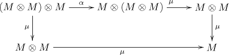
In this case, M is a category; think of it as a fixed but arbitrary class, e.g., ValidationResult or Node. As programmers, we operate on instances of those classes but ignore that for now
On the first line, we have three terms; let’s index them 0, 1, and 2. On the bottom line, we have two terms; index 3 and 4. In between these terms, we have arrows, which are transformations.
1->2: we see that \(\alpha\) is association where we move the parenthesis around. We introduced associativity as a property of a monoid earlier.
2->3 we see that we have “reduced” the equation \(M \bigotimes (M \bigotimes M)\) into \(M \bigotimes M\) by applying \(1 \bigotimes \mu\), which is equivalent to saying that the first term (the M not in the parens) is the identity. We can do this because monoids must have an identity.
2->4 is the same as the above, but with the parens in a different location
4->5 && 3->5: is the result of just evaluation the x, the \(\mu\).
And there you go!
Closing Thoughts
This post came about after a discussion with one of my mentees. That mentee was facing something similar, and as someone who has gone through this EXACT problem, I thought I’d write about it and share what I’ve learned.
Also, I firmly believe that one way to ensure you know something is by explaining it. And so, to finally understand what
A monad is a monoid in the category of endofunctors, what’s the problem?
I’ve decided to write a 3-part series on “What is a monoid?”, “What is an endofunctor” and “What is a monad”. All those posts will build off one another so stick around!
]]>